When I first made the python version of the net worth spreadsheet, I used a function like this:

def netWorthByAge(
    ages, 
    savingsRate = 0.18, 
    startingNetWorth = 10000,
    startingSalary = 40000,
    raises = 0.025,
    
    marketReturn = 0.06,
    inflation = 0.02,
    
    retirementAge = 65
  ):

You could pass in parameters, but only constants. This is how the spreadsheet works as well—each cell contains a constant.

The first thing to do to make it more flexible is to use a lambda instead for the marketReturn parameter:

marketReturn = (lambda age: 0.06),

Then, when you use it, you need to call it like a function:

netWorth = netWorth * (1 + marketReturn(age - 1)) + savings

We use last year’s market return to grow your current net worth and then add in your new savings.

The default function is

(lambda age: 0.06)

This just says that 0.06 is the return at every age, so it’s effectively a constant.

But, instead, we could use historical market data. You can see this file that parses the TSV market data file and gives you a simple function to look up a historical return for a given year.

Then, I just need to create a lambda that looks up a market rate based on the age and starting year:

mktData = mktdata.readMktData()
for startingYear in range(fromYear, toYear, 5):
  scenario = networth.netWorthByAge(ages = ages,
    savingsRate = savingsRate, 
    marketReturn = (lambda age: mktdata.mktReturn(mktData, age, startingYear = startingYear))
  )

And this will create a scenario (an array of doubles representing net worth) for each year in the simulation.

You can download and run the code to play with it. Here’s a sample chart it generates:

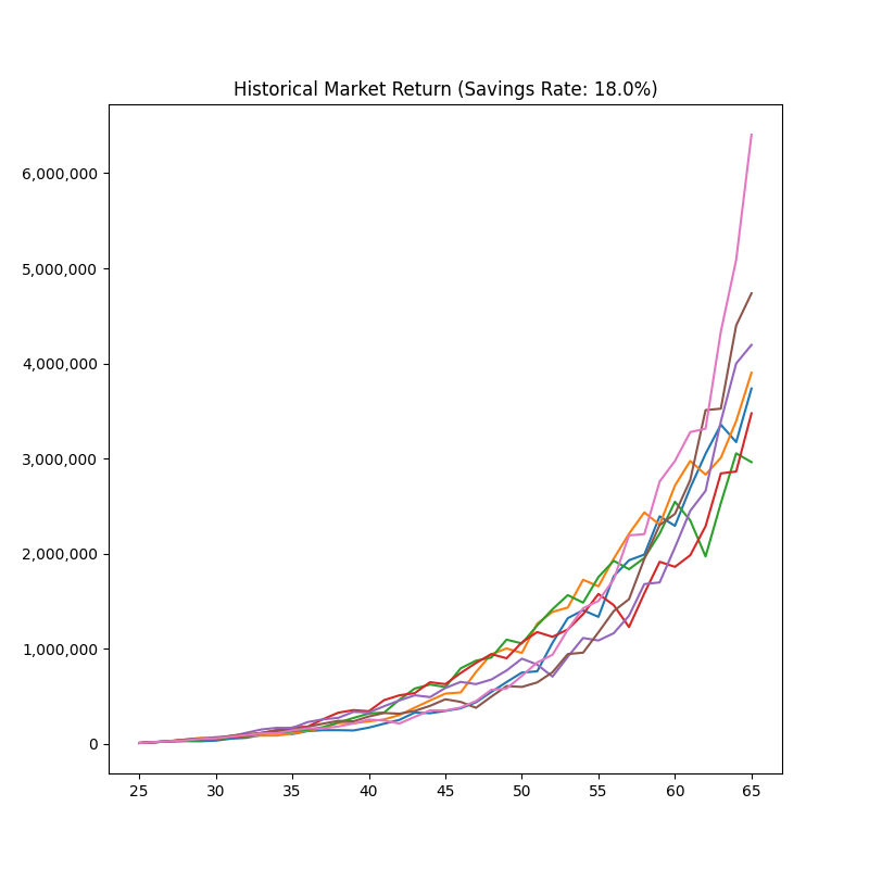
There are lines for starting the simulation in 1928, 1933, 1938, 1943, 1948, 1953, and 1958. This gives you an idea of the expected range of possibilities.